Data Masking Algorithm Strength
Slide 1
In our prior webinars, we have covered different aspects of the data development lifecycle and SSIS. They are listed here on the slide:
Prior Webinars included:
SSIS-first experience;
Lifecycle;
Testing with SSIS;
ETL vs ELT.
Data Masking Algorithms, among them: Substitution, Shuffling, Random, Date aging (AKA Number and Date Variance), Encryption (specifcally, tokenization), Nulling out or deletion, Value changes in increments or decrements, as well as Custom algorithms
Slide 2
We have looked at the scenarios involving data masking in different environments as they pertain to different insiders threats based on roles. We implemented a simple lifecycle. We did some test cases in SSIS including regression testing, and showed advantages and disadvantages of ETL (extract-transform-load) vs ELT (extract-load-transform).
Slide 3
We gave a definition of data masking:
Obfuscating sensitive data elements with “false” values within a data store while preserving data look, feel, and usability in applications.
Slide 4
We listed all the algorithms and showed examples of their implementations. Some algorithms are very simple and fast to implement, while others are very complex and allow for a lot of protection. We have shown two very different algorithms: a simple shift, versus a Format-Preserving Encryption that involves multiple cycles, yet due to its strength it is very difficult to hack. Among algorithmic features, the most important for data masking is the strength of the algorithms from the security standpoint.
And today we do a deep dive and explore two of the most common algorithms in detail. Often times, in order to protect, we first need to understand how to break in – so we take a “think hacker” approach, explore a couple of ways to “break” the system, and show you how a well-chosen algorithm could protect your data in each scenario.
Slide 5
In order to better understand how we secure data, we first need to understand the properties of data while it is stored. The very first thing to understand is the fact that some data is unique and some is not. Data models a physical world. In a physical world, each person is unique, yet all of us have repeating attributes: almost all of us are one of two genders, with outliers being such a small percentage of the total population that statistically, you can assume approximately 50% of a given sample is one and 50% is the other. We all have names and we all have age and we live somewhere – and these “properties” are not unique. Many more people live in New York than in Aspen. There are many more Janes than Virginias. These statistical distributions are a powerful thing. The most famous example of a “hack” based on statistical distributions grew out of research from a graduate student named Latanya Sweeney from Carnegie Mellon University. Latanya linked the anonymized GIC database (which retained the birth date, sex, and ZIP code of each patient) with voter registration records to identify the medical record of the governor of Massachusetts, and later created the whole field of computer science and math which deals with the so-called differential privacy. The essence of the case is reflected in the slide. Latanya found that only six people in Cambridge shared the governor’s birth date, only three of them were men, and of them, only he lived in his ZIP code. Making further calculations, Latanya defined that 87 percent of all Americans could be uniquely identified using only three bits of information: ZIP code, birth date, and gender.
Slide 6
The threat is well recognized, and on top of many privacy laws in many industries such as GLBA in the financial industry, FERPA in education, and many state laws, as well as HIPAA, the Department of Health and Human services published a guide on its site on how to de-identify sensitive data. It's a “Safe Harbor” for making sure statistics are enforced in several elements, including zip code and dates. It does not mean that we should not take more protection, just these are the minimum requirements that people have to be aware of when masking data.
Slide 7
Let’s start now on the algorithms – and explain the reasoning in several very simple examples.
Slide 8
The first algorithm we will consider is shuffling. In Shuffling, the data is shuffled within the column. No data is replaced per se, just the index in the column changes. In some sense, people define shuffling as a substitution with mapping to its own set of data. This algorithm is great for maintaining aggregates. An example application is when you need to maintain the end of year sales figure.
Different algorithms are used for shuffling. The simplest one is shifting records along with the same number. Let’s consider an example.
Slide 9
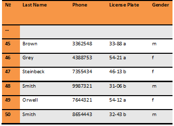
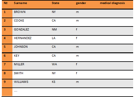
Let's say we have a database of voters. For simplicity's sake, we will examine a simple table with columns and rows. It has fields with unique values (license plate and phone number of the car), and repetitive values (such as name and gender). The example shows only the last few lines of the table.
After we mask data and move it to the development environment, the masked database has the same number of rows, N = 50, and looks like this: +4+3+2
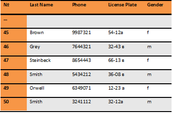
Please note that we employed a different shift for different columns, +4 for the phone, +3 for license plates and +2 for gender.
Someone attempting to hack this algorithm would try to use data from the second, masked, table to restore the values in the first, the production table.
Slide 10
One of the ways to do this is to enter a row with some unique traceable data - let’s say a name - into the production table. Again, for simplicity, we assume in this example that the name does not shift. It should be noted that choosing a plausible unique name is not difficult, for example, by changing one letter in the last name (since in real life there are no last names like the name “Smith” spelled with two ts or two hs).
Now, let's consider the scenario when a hacker adds such a record into initial database: a row defined by new name, Smitth
The initial production database with the new name added, so the number of records is N = 51 , looks like this:
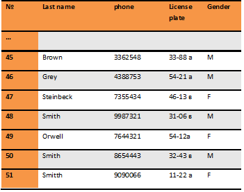
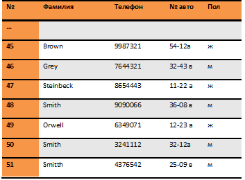
After the masking cycle, we get the following database data set in production:
Data Base with masked data, N = 51
According to Table 4, the shuffle for unique data (phone number, and a car) is easily defined.
Slide 11
In the case of gender, it would be impossible. The probability of a correct correspondence between name and gender depends on how many are women there are in the table (an original set for women). Since we are interested only in the correct sequence of the Gender column, then the probability of being a woman is
P = 1 / number of women.
If the hacker knows how many women and men are originally in the table, he will insert a record with the gender that has fewer entries.
Suppose in our example the basis is 20 women (20 letters f in Tables 1 and 2 in the column Gender) Then the probability of full recovery of the data set for the gender is
P = 1 / (number of women + 1) = 1/21.
Security in data masking is all about the probability of de-identification. As we can see, Simple Shuffling is not a very secure algorithm; however, adding complexity to the shuffling algorithm will yield better results.
Slide 12
Now, let’s consider another algorithm that is also often used in data masking – substitution. Substitution is an algorithm in which another authentic looking value can be substituted for the existing value. It is best suited for non-unique data. This is also an algorithm most often mentioned in the open source community. Here are the two blogs that we mentioned previously: substitution for unique social security number:
https://www.mssqltips.com/sqlservertip/3091/masking-personal-identifiable-sql-server-data/
Substitution for non-unique names:
https://www.brentozar.com/archive/2011/09/how-do-you-mask-data/
Slide 13
Let’s consider the latest example. In order to maintain the mapping table, you will have to get a distinct data set of names from production and create a mapping table that maps values one to one. The author does acknowledge in the blog that security is not enforced to the fullest. But how strong will be such a method be?
Slide 14
Consider the following case. We want to determine the possibility of the correct diagnosis of a particular person in the database, presented in part in Table 1. We are assuming that the data in the database are collected throughout the United States and are represented proportionally (ie, no female-dominated diseases, or diseases specific to the State of Alaska). In this case the data set is a representative sample of the patients. We believe that the database has 10,000 patients (or rows).
Slide 15
For masking data purposes, we replaced all the names in a one-to-one manner. For example:
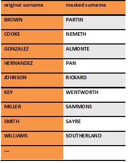
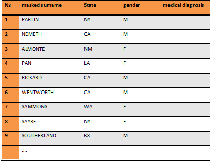
Now, after we masked the data based on mapping these substitution values, let's look at the resulting table
Slide 16
Suppose you want to discover the diagnosis of your colleague JOHNSON and neighbor SOOKE as you want to know whether your colleague's disease is terminal (so you'll finally get that promotion) and whether your loud neighbor SOOKE will lose his voice forever and stop keeping you up all night.
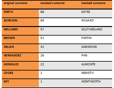
To do this, you implement a frequency analysis of last names. Using, for example, the site https://probablyhelpful.com/ you can see frequencies of the most common American last names. Since the sample of 10,000 is large enough, most frequently used names will be absolutely guaranteed to occur in the appropriate proportions in the data set. Since the names are masked in a proportion 1:1, new, substituted names will have the same frequency of occurrence:
Slide 17
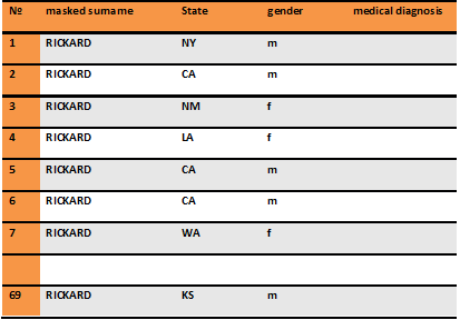
I.e. the frequency of a substitution for the last name JOHNSON will coincide with the frequency of last name JOHNSON in the original set. And, based on the data frequency table of the above-mentioned site, it will be the second most frequent name. Obviously, this name is RICKARD.
The instance of this name in the database with 10,000 data points will be approximately 69:
Slide 18
Your chance to correctly establish the diagnosis is then 1/69 (assume all diagnoses are unique).
Let's say you know a small amount of statistical information about the data set, that all the addresses are located in the United States. If you pick a state, for example, CA, you can use some statistical information to further re-identify the data set. According to the 2011 Census, population in California is approximately 38 million people. The United States has, total, approximately 310 million people. The probability that a person in the database is from California is therefore 38/311 or 0.122. Therefore, approximately 12% of the 69 instances of RICKARD will be Californian, or about 8 people. The probability of guessing correctly is now 1/8.
Knowing that JOHNSON (masked as RICKARD) is a man, on the basis of approximately an equal ratio of men and women, we find that the probability of a correct diagnosis of the situation described is 1/4.
If the last name is uncommon, for example SOOKE, the chances of guessing are greatly reduced. In this case, it is impossible to ascertain the proper name of SOOKE in the new table.
Using the table of the frequency of last names (out of 100,000) from the site, we can determine the total percentage of names that occur less than 2 times in 10,000 values. This corresponds approximately to the uncommon last names, all names (like SOOKE) that are more rare than HOUSE (and HOUSE only occurs 15 times in the 100,000). Therefore, it will be assumed that all the names on the list below HOUSE in a 10,000 item list meet at least 2 times. The cumulative percentage of last names less common than HOUSE are approximately 37.5% (or 37594.06 out of 100,000). Thus, any uncommon, single last name in a database of 10,000 values will occur in 62.5% of those values.
Your chance is now 1/6250.
If you know the information about the place of residence - State of California, then the names of 6250 will be approximately 12% of Californians, ie 750 people. The probability of guessing is 1/750. Knowing that SOOKE is a man, we find that the probability of a correct diagnosis of the situation is approximately 1/375.
Slide 19
Probabilities increase when we don’t do 1:1 substitution and increase the disturbance in statistics. There is a lot of work being done in this area in different research labs at major universities, at Microsoft and other companies. We translated this research into the product - so that you don't have to.


